Training a neural network for image recognition.
Training a neural network for image recognition.
1st of February 2018

Summary
This blog post describes how to create a neural network to recognize clothing pieces in pictures provided by Zalando. This post is written for very beginners and R users. Just here to check out the code, click here.
- Keywords: Deep learning, multinominal classification, neural network, image recognition.
- Level of programming: Beginner
- Programming language: R
- Reading time: 10 min
Introduction
Machine-learning technology powers many aspects of modern society: from searching on the web to recommendations on e-commerce websites, and it is increasingly present in consumer products. Increasingly, these applications make use of a class of techniques called deep learning. Building a neural network is a form of deep learning. Deep learning also has shown promising results in natural language understanding, topic classification, sentiment analysis, question answering and language translation (Lecun, Bengio & Hinton, 2015; Krizhevsky, Sutskever & Hinton, 2017).
Neural networks
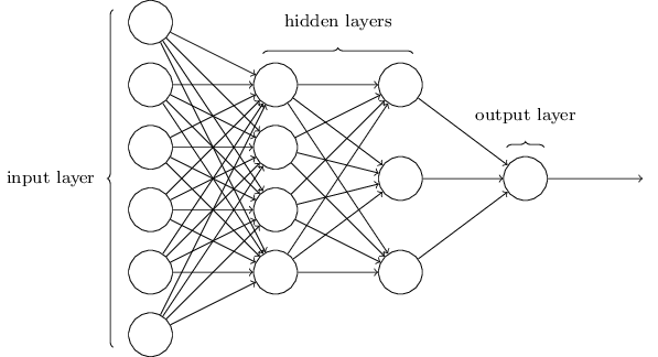
Lecun, Bengio & Hinton (2015) describe a training technique: the backpropagation algorithm. In figure 1, we feedforward the input to a prediction and backpropagate the error to update the weights.

Figure 1, a neural network.
Input layer
A neural network is created by training an algorithm to discover structure in a dataset. The network is shown an image and produces an output in the form probability scores, one for each category/label with an unnormalized softmax activation function. The desired category should have the highest scores of all categories, which is very unlikely to happen before training (Lecun, Bengio & Hinton, 2015). For example, when the input is a picture of a t-shirt, the machine should assign the highest probability to the category t-shirts.
Hidden layers
The network computes an objective function which measures the error between the output scores and the desired scores. The machine then modifies its adjustable weights to reduce this error. These weights are numbers that can be seen as “knobs” that represent the input-output function of the total network. For each “knob” the machine learns by what amount the error would increase or decrease if the weight where increased by a tiny amount. This process continues to happen until the machine finds the lowest total error possible. Therefore, the algorithm is able to take an input and produce the best output possible based on the training data (Lecun, Bengio & Hinton, 2015).
If you want to dig deeper and really want to understand the mathematical way of calculating the weights, I would recommend this article by Yann LeCun. Or for a brief gist, you could watch this video about deep learning.
Let’s build our own neural network
The main advantage of a neural network is the ease of programming one. An important part is having a good dataset. Let’s take a shot with data from a clothing retailer Zalando.
The dataset of clothing images from Zalando
 Figure 2, dataset of Zalando loaded in R.
Zalando provided a dataset of 70.000 clothing images. The training and test datasets have 785 columns. The first column consists of the class labels (see below), and represents the type of clothing.
- 0 - T-shirt/top
- 1 - Trouser
- 2 - Pullover
The rest of the columns contain the pixel-values of the associated image. Each pixel has a single pixel-value associated with it, indicating the lightness or darkness of that pixel, with higher numbers meaning darker. This pixel-value is an integer between 0 and 255. An example of the dataset can be found here.
Data manipulation
To train and test the neural network use the neuralnet library. Furthermore, data.table to read the Zalando data and dplyr for data manipulation.
library(neuralnet)
library(data.table)
library(dplyr)
Reading the data
To collect the data from Zalando, you can download from their website and load the data into R with the fread() function from the data.table package. Zalando already divided the data into a train and test file. However, this may not be the ideal set up. Therefore, the data is combined in the fashiondata object, with the rbind() function.
fashion_train <- fread("C:/Users/Gilia/Documents/fashion_train.csv")
fashion_test <- fread("C:/Users/Gilia/Documents/fashion_test.csv")
fashiondata <- rbind(fashion_test, fashion_train)
Because the dataset contains numerous images, it is recommended to build your first neural network on a couple of labels and gradually add more labels/data. In the next piece of code the total dataset is filtered on the first three labels (0, 1 and 2) and with the str() function check whether the data is filtered correctly.
fashiondata <- fashiondata %>% filter(label == 0 | label == 1 | label == 2)
str(fashiondata)
In this case, there are no missing data points. If there would be missing data points for the pixels, you could delete the image completely. Make sure you check this for your dataset. Otherwise, your neural net won’t work.
Standardization of the data
By standardizing the data before you fit your neural network, the process of fitting the neural network will go faster (Sola & Sevilla, 1997). There are numerous ways of standardizing the pixel scores of the dataset: min-max standardization, z-score standardization, etc. In this case, min-max standardization will do, because it retains the original distribution.
First, remove the actual label column from the dataset because the label should not be standardized along with the actual pixel scores with fashiondata$label <- NULL . Save the label column into a separate dataframe for later manipulation label <- fashiondata$label.
Next up, the data gets normalized. Which transforms the original pixels to a score ranging from 0 to 1.
maxs <- apply(fashiondata, 2, max)
mins <- apply(fashiondata, 2, min)
scaled <- as.data.frame(scale(fashiondata, center = mins, scale = maxs - mins))
Create dummy variables
The dataset only contains one column where it says whether it is a t-shirt (0) or a trouser (1) or a pullover (2). To let the neural network to calculate probabilities for each category, create a dummy variables from this column. By transforming the label column into this format, the neural network can calculate the probability for each category separatly.
# Encode as a one hot vector multilabel data
labels <- cbind(label, class.ind(as.factor(label)))
This means transforming your data from this:
| Label |
|---|
| 0 |
| 1 |
| 2 |
To this:
| 0 | 1 | 2 |
|---|---|---|
| 1 | 0 | 0 |
| 0 | 1 | 0 |
| 0 | 0 | 1 |
Combining the labels and normalized data
Now that the data is normalized and the dummy variables are created, combine them into a single dataframe.
colnames(labels) <- c("label", "l0", "l1","l2")
fashiondata <- cbind(labels, scaled)
By now your fashiondata dataframe consists out of the correct labels and normalized pixel data, as in figure 3.

Figure 3, example of your dataframe by now.
Random sample the test and training data
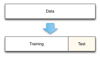
When your data is complete it is time to divide your total data into a training set and test set. From this training set the model is derived. From the test set it is possible to “test” the accuracy of the model. This process is visualized in figure 4.

Figure 4, the flow of building a neural net.
In this case, the training data consist out of 90% of the total data. Whereas, the test data is only 10% of the total data. It is crucial to note when data splitting, the issue is not about what proportion of data should be allocated in each sample. Rather, it is about sufficient data points in each sample to ensure adequate learning, validation, and testing (Zhang, 1997).
samplesize = 0.90 * nrow(fashiondata)
index = sample(seq_len(nrow(fashiondata)), size = samplesize )

# Creates training and test set
fashion_train = fashiondata[index,]
fashion_test = fashiondata[-index,]
Also, the label column is still in the test and training dataframe. This label is deleted from both datasets as it no longer functions as an input for our neural net.
# remove label from training and test data
fashion_test$label <- NULL
fashion_train$label <- NULL
One more step before the magic happens
Before the neural net can be trained and tested, it is recommended to check whether all the previous procedures of data manipulation and cleaning all went correctly. To check if the scaling and sampling worked correctly, the function str() shows the structure of both datasets.
# check if label is removed and scaling and sampling worked
str(fashion_train)
str(fashion_test)
Training the neural network

Now if all the previous steps went correctly, we arrive at the exciting part of this blog post. First of all, the following code creates the formula for the neural network. Our goal is to predict what type of clothing the pixels match to so, l0, l1 and l2 are our y variables (output). The pixel columns ranging from 1 to 784 represent the x variables (input).
# neural net formula
n <- names(fashion_train)
f <- as.formula(paste("l0 + l1 + l2 ~", paste(n[!n %in% c("l0", "l1", "l2")], collapse = " + ")))
This piece of code gives us the following formula to feed the neural network l0 + l1 + l2 ~ pixel1 + pixel2 + pixel3 + pixel4 + pixel5 + pixel6 ... pixel784.
Fit your neural network
Next, the neural network gets fit over the data according to the formula with the following piece of code.
neuralnetwork <- neuralnet(f, data = fashion_train, hidden = 2, linear.output = F)
f: The formula object.
data: The training dataset that is used to train the model on. The formula needs to be corresponding to the column names of the training dataset.
hidden: The number of hidden layers. There is not really a perfect way to determine the “right” amount of hidden layers. In this case, two hidden layers will do the job. It is up to you to experiment, what number of layers will get a more accurate model. Remember that when adding more hidden layers, the network takes more time to train.
linear.output: If the model is a linear model. In this case we try to classify the pixels in a label. Therefore, the parameter is set to FALSE.
This process may take some time. Get ready to make a cup of coffee or tea, as this process may take up to 5 hours.
Neural network
To see your created neural network, use the function plot(neuralnetwork). This will result in a graphical representation of your model (input, hidden layer and output), the calculated weights and biases.

Figure 5, our neural network
The inputs are the pixel variables as indicated in our formula, that take values from 0 to 255, as specified in our dataset. The lines from the input layers direct to the hidden layers. Where the weights are calculated for all 784 pixels. These weights point towards the output where, depending on the input, a probability score will be calculated for each category.
Predict over the training set
Now that the model is created over the data. It is time to check whether our model is actually good at classifying the pixels into clothing categories.
With the function compute() from the neuralnet package it is possible to predict over the test data what type of clothing piece it is, by the pixel combination. In the code it is important to exclude the actual labels, this data gets excluded by using fashion_test[, 3:786]. The neural network calculates the probabilities for all categories and saves it in the object pr.nn$net.result. The probabilities are saved in results in the second to last line of code. The last step is to round up the probabilities towards 1 or 0.
# predict for test data
pr.nn <- neuralnet::compute(neuralnetwork, fashion_test[, 3:786])
pr.nn$net.result
results <- as.data.frame(pr.nn$net.result)
results <- round(results)
This results in a dataframe as displayed below.

Figure 6, the results of the neural network
Looking at figure 6, the neural network decided that image 4 of the test data is a pullover. Let’s examine the accuracy of the model over all the test data.
Accuracy of the neural network
The accuracy of the model is calculated by taking the truth (the actual test data), and the predicted values by the neural network (results). With the function mean() the values of both points of truths are compared and give us a percentage of correctly predicted images (Zhang, 1997).
# get the column with highest probability
original_values <- max.col(fashion_test[,1:3])
test_values <- max.col(results)

# calculate accuracy
mean(test_values == original_values)
This neural network predicted 87% of the images correctly. This makes this neural network actually quite powerful. A score of 100% would be considered an overfit, as the model would be almost “resistant” towards big changes in the data.

References
Krizhevsky, A., Sutskever, I., & Hinton, G. E. 2017. ImageNet classification with deep convolutional neural networks. Communications of the ACM, 60(6): 84–90.
Lecun, Y., Bengio, Y., & Hinton, G. 2015. Deep learning. Nature, 521(7553): 436–444.
Sola, J., & Sevilla, J. 1997. Importance of input data normalization for the application of neural networks to complex industrial problems. IEEE Transactions on Nuclear Science, 44(3): 1464–1468.
Zhang, G. P. 1997. Business Forecasting with Artificial Neural Networks. Neural Networks in Business Forecasting, 35–62.